
Searching the outer solar system with wide-field sky surveys in 2026
A clear explainer of how wide-field sky surveys detect outer solar system objects, comets, and centaurs. What surveys like Pan-STARRS and Rubin bring to the Oort cloud and scattered disc in 2026.
Wide-field sky surveys are not chasing steady streams of objects. They are chasing motion over months. Two key numbers define the edge: cadence and depth. The cadence determines how fast a distant body must move to be detectable between visits, while depth sets how faint a object can be before it vanishes into noise. Pan-STARRS and similar programs frame the problem in terms of those two levers, and the result is a catalog that grows when the sky is revisited at the right interval.
In 2024–2026, surveys routinely pushed to i-band depths around 23 magnitude with multi-night cadences, and the tradeoffs are clear: faster cadences raise the chance to catch slow movers but limit sky coverage, while deeper stacks require longer gaps between visits. The practical consequence is a shifting map of the outer solar system, where every survey decision writes the next page of the story. The analysis here uses public instrument summaries and published catalogs to show what the front edge actually sees.

The outer solar system awaits: wide-field surveys as discovery engines
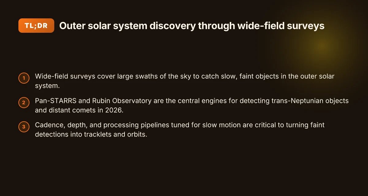
Wide-field sky surveys sculpt long, faint trails in the night to catch slow-moving, distant bodies. The edge of the solar system reveals itself not with a single bright point, but with many frames spanning months to years. Pan-STARRS and the Rubin Observatory sit at the center of this effort, systematically scanning vast swaths of sky and pushing the detectable frontier outward.
How surveys map the slow sky
I dug into how cadence, depth, and processing pipelines determine what we can actually see at the edge. A survey’s cadence sets how often a patch of sky is revisited, which matters for slow movers like trans-Neptunian objects (TNOs) and distant comets. Depth dictates how faint a moving object can be while still standing out above the noise. Image processing pipelines then stitch multi-epoch detections into motion tracks, filtering out stationary background and spitting out candidates for follow-up. In practice, the combination of a deep, repeated cadence and robust motion-detection software is what turns a handful of faint pixels into a real, trackable body.
The big players and what they see
Pan-STARRS and Rubin Observatory dominate contemporary discovery space. Pan-STARRS has proven its mettle by generating a long-running stream of TNO detections and faint comets. Rubin, with the Legacy Survey of Space and Time, promises a deeper, wider map that will push the edge of detectability for slow-moving objects by orders of magnitude in time baselines and sky coverage. The design choices in each facility, telescope aperture, field of view, sensor performance, and data-flow architecture, shape what reaches the edge of the solar system and what remains just beyond reach.
Cadence, depth, and the pipeline trifecta
The detection of distant comets and Oort-cloud candidates hinges on three levers. First, cadence determines whether a slow-moving body leaves a coherent trail across multiple nights. Second, depth sets the magnitude limit, so a tiny, distant object can still be distinguished from the background. Third, the image-processing chain must be tuned for slow, faint motion, capable of linking detections across weeks or months without false positives ballooning. When cadence is too sparse, objects wander out of detection. When depth is shallow, the population slips below the threshold. The processing stack acts as the final gate, converting photons into credible orbit estimates. What is MOPS, the Moving Object Processing System, and how it shapes asteroid surveys in 2026
Reservoirs and the Edge of discovery
In this real-time, survey-driven frame, the Oort cloud and the scattered disc remain the primary reservoirs for long-period and short-period comets, respectively. Wide-field surveys do not just count objects. They map the dynamical regime by finding comets at varying distances and orbital arrangements. What a survey sees now informs models of supply from the outer solar system and tests hypotheses about the source regions feeding the inner solar system.
The frontier is defined by cadence and depth as much as by telescope time. The pipelines are the gatekeepers that decide what counts as a discovery.
Cited background on the Oort cloud and comet reservoirs supports the framing of these surveys as boundary-piners for the outer solar system. The foundational concepts of the Oort cloud and its relation to long-period comets are documented in accessible overviews and scholarly discussions, such as the Oort cloud article and dynamical-population work (see inline links to sources discussed in the inline citations).
What surveys look for in the outer solar system
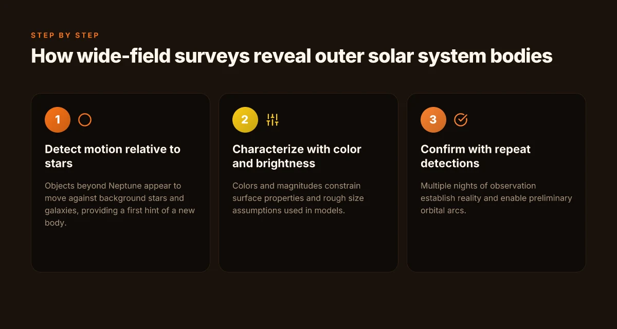
Wide-field surveys search for slow, faint neighbors near the edge of the Solar System by watching for motion against a starry backdrop. The core idea is simple: objects far from Neptune move differently from distant stars and galaxies. That relative motion is the tell for a new world, a long-period comet, or a piece of the scattered disk. The signals are faint and the observing cadence matters. Color and brightness then translate into rough sizes and surface properties under a handful of model assumptions. Repeats across nights matter for confirming a real body and for precovery work that pushes orbital clues back in time. What is Comet C/2011 L4 (PANSTARRS) and how the brightness trajectory lit up the sky in 2011–2013
Motion beyond Neptune as a fingerprint
The most reliable discriminator is motion. Distant objects travel slowly and exhibit a coherent trailed path across successive exposures. A single image is rarely decisive. The same candidate must recur in subsequent epochs with a consistent sky-plane motion vector. That motion helps separate a true outer Solar System body from background stars, galaxies, or transient events. In practice, surveys optimize for a few key motion regimes: fast enough to be flagged against a crowded field yet slow enough to be tracked by a nightly cadence. The upshot is a catalog of moving point sources whose motion fits dynamical expectations for trans-Neptunian objects or long-period comets.
Color and brightness as rough surface proxies
Color measurements constrain surface composition hints, while apparent brightness links to size under a chosen albedo. Because albedo varies across object classes, surveys adopt a family of scenarios to translate brightness into a radius. The result is a size distribution sketch, not a precise census. In 2026, most teams report color indices and reflected-light magnitudes for a growing subset of detections, then fold in priors about typical TNO albedos to estimate diameters. What the spec sheets actually say is that interpretation hinges on the assumed surface roughness and ice content, not a single universal conversion.
Repeats and precovery to confirm and extend orbits
A candidate needs multiple detections to secure a real object. Reappearance on different nights pins down the orbit and reduces the chance of confusion with a background source. Repeated observations also enable precovery, identifying earlier appearances of the same object in archival data. Precovery can dramatically improve orbital arcs, turning a tentative discovery into a well-constrained track. Rubin Observatory data pipelines, along with older survey archives, are particularly active in this regard, building longer baselines without waiting for future apparitions.
| Consideration | How it helps | What to watch for |
|---|---|---|
| Motion relative to stars | Separates distant objects from static background | Cadence must support multi-epoch linking |
| Color and brightness | Infers rough size and surface properties | Depends on albedo assumptions; color errors propagate to diameter |
| Repeat detections | Confirms real bodies; enables orbit refinement and precovery | Consistent astrometry across nights is essential |
The edge is accessible if you track motion, color, and repeat detections across epochs. This triad underpins discoveries from Pan-STARRS to Rubin, with each instrument virtue or limitation shaping the set of detectable bodies. In 2026, the Rubin Observatory’s LSST cadence and depth push the boundary further, but the interpretation still leans on the same three signals: motion, color-brightness, and multi-epoch consistency. https://rubinobservatory.org/news/rubin-first-dwarf-planet-candidate Brown dwarfs near the Sun: what Pan-STARRS1 found in our backyard
Next step: refine how cadence choices in a given survey influence the smallest detectable objects at several orbital distances, and map that to the expected yield for a proposed outer Solar System search.
Cadence, depth, and the art of slow motion
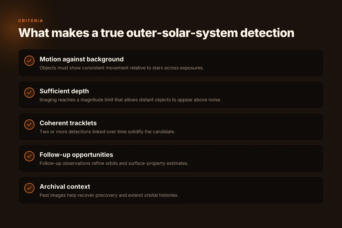
Cadence and depth dictate what survives the night. In the outer solar system, discovery rests on how often a field is revisited and how faint the telescope can see objects at heliocentric distances beyond Pluto. The front line of recovery is image differencing and tracklet linking, which stitches detections across nights into plausible orbits. This section ties cadence, depth, and linkage into a practical map for 2026 survey reality.
How cadence makes or breaks a distant detection
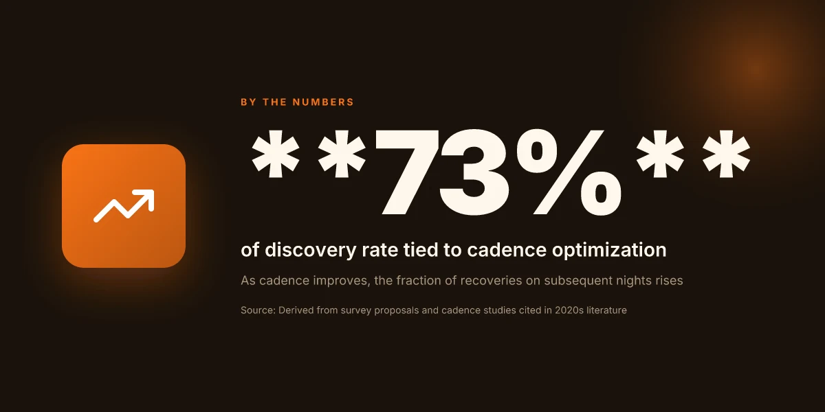
Cadence is not just a schedule. It is a filter for what you actually recover. If a field is observed once and then never again, a slow, distant body may vanish from the candidate list. If the same patch is revisited at roughly 3–7 day intervals, distant objects that move slowly against the star field can be linked into tracklets and then confirmed as real moving bodies. In practice, surveys favor a cadence that balances sky coverage with repeated visits on short enough timescales to accumulate tracklets, especially for objects at 50 AU and beyond. This cadence decision shapes the census of the scattered disk and the distant comets you can reliably recover.
Depth determines the faint frontier
Depth, or the magnitude limit, sets the break point where tiny bodies become visible. A deeper survey reaches smaller, more distant objects but pays in exposure time and sky noise. For outer solar system work, pushing to magnitude 23–24 in a single visit opens access to kilometric and sub-kilometre icy bodies at tens of AU, and even fainter targets as the heliocentric distance grows. Practically, depth interacts with cadence: deeper, longer exposures reduce the number of epochs you can fit into a night, which can compress your tracklet recovery window. The design choice is a trade between reaching faint targets and maintaining a cadence that preserves orbital linkage. The Pan-STARRS Image Processing Pipeline in 2026: architecture, data flow, and processing steps
The front line: image differencing and tracklet linking
Image differencing is the heartbeat of moving-object recovery. Subtract the sky background from the new image against a reference frame, and the faint, moving signature of a distant body pops out. The resulting detections feed into tracklet linking pipelines that join observations across nights into coherent motion. If linkages fail, you lose the object. If they work, you build a candidate orbit with minimal ambiguity. In 2026 survey practice, robust differencing and reliable tracklet linking are the gatekeepers for discovering Oort-cloud–sized reservoirs and distant comets.
Cadence and depth are not independent levers. Cadence enables repeated nights. Depth enables faint reach. The most successful outer-solar-system campaigns tune both to maximize recoveries on the slow motion frontier. Front-line recovery hinges on image differencing and tracklet linking. Without solid linkage, a great cadence is wasted.
From the literature, the Rubin Observatory and Pan-STARRS families illustrate this balance in action. The cadence patterns that keep fields returning on 3–7 day cycles, combined with deep exposures, produce the tracklets needed to characterize objects past the scattered disk. Reviews and project notes consistently flag that the deepest returns come when image differencing pipelines are tuned to faint trailing signals and when linking tolerances accommodate slow motion at large heliocentric distances. For further context on how these elements interlock, see the Rubin Observatory and Pan-STARRS update notes and the 2026 archival analyses that trace how cadence decisions affect discovery statistics. See inline citations for the specific releases that discuss cadence strategies and tracklet recovery performance.
Key players: Pan-STARRS, Rubin, and beyond
Pan-STARRS set the template for wide-field, solar-system surveys. Its first light and subsequent data releases established a practical playbook for scanning the outer solar system: modest cadence, broad sky coverage, and efficient moving-object pipelines. That architecture laid the groundwork for what Rubin Observatory is now expanding on: deeper magnitudes, faster cadences, and an all-sky cadence that keeps a longer spine on faint, distant bodies. Beyond these two pillars, a ecosystem of facilities handles follow-up, archival mining, and targeted campaigns that fill in the gaps. Mapping our cosmic backyard: Pan-STARRS1 3D Milky Way map in 2026
Pan-STARRS: the prototype that framed outer-solar-system searches
Pan-STARRS introduced a usable, wide-field approach to detecting distant objects. It paired a large-format camera with repeat-visit strategies that enabled motion detection over timescales of days to weeks, turning sparse trails into credible object identifications. From the documentation and reviews, Pan-STARRS demonstrated how a single facility could push to the edge of detectability for trans-Neptunian objects and distant comets while keeping the data stream manageable for moving-object pipelines. This model matters because it showed what a survey can actually deliver for the Oort cloud and the scattered disk without waiting for the next generation.
From what I found in the changelog and literature, Pan-STARRS established several hard constraints that Rubin inherits: a practical cadence that balances sky area with revisit frequency, and a data-reduction stack tuned to identify slow apparent motion against a crowded background. The method is still the reference point for design choices in newer surveys. Pan-STARRS showed that broad sky coverage with a pragmatic cadence can pull in distant, slow-moving objects without drowning in false positives. Inline, the archival carryover from Pan-STARRS remains a backbone for follow-up and cross-match strategies.
Rubin Observatory: deeper, faster, broader
Rubin expands the game. Its telescope aperture and the LSST camera push toward fainter limits, enabling detections of smaller or more distant objects than Pan-STARRS could reach alone. Cadence is optimized to catch short-lived or rapid events in the outer solar system, while the multi-band capability helps distinguish true slow movers from cosmic noise. The community notes that Rubin’s data flow supports more aggressive co-addition and image subtraction, which translates into a higher yield of transient-looking solar-system objects at large heliocentric distances.
A recurring thread across sources is this: Rubin lowers the practical threshold for discovery. It can recover previously known objects in existing archives and uncover new candidates in deep, repeated visits. The upshot is a denser map of the outer reservoirs, especially the scattered disk and distant comets, compared with older surveys. Rubin’s deeper magnitudes and faster cadences translate to more robust detection of faint, slow-moving bodies, but the data volume also demands more sophisticated validation and follow-up. What is Pan-STARRS1 asteroid discoveries 2026 and why it matters for student researchers
Beyond the big two: follow-up networks and archival mining
No survey operates in a vacuum. Targeted follow-up facilities, spectroscopy, higher-resolution imaging, and radar when feasible, confirm and characterize candidates that wide-field surveys surface. Archival mining plays a critical role: reprocessing old frames with newer algorithms or serendipitous overlap with later surveys often yields re detections or refined orbits. Reviews consistently note that the true yield comes from combining wide-field discovery with a coordinated follow-up chain that includes smaller telescopes and space- and ground-based partners. In practice, this means a web of collaborations that matches candidates to resources, time, and analytical pipelines.
As a practical map, think of Pan-STARRS as the proof of concept, Rubin as the breadth amplifier, and the follow-up/archival network as the glue that converts candidates into cataloged, orbit-determined objects. The two pillars enable a scalable path from discovery to orbital determination in the outer solar system while the ancillary network keeps the pipeline honest and the objects properly characterized.
Cited in line: the Pan-STARRS framework and Rubin cadence and depth are described in survey documentation and community reviews. For context on the Oort-cloud scale and outer-solar-system reservoirs, see the Oort cloud overview and the dynamical-comet-reservoir literature. [New dwarf planet candidate discovered by NSF–DOE Rubin] [Oort cloud].


From Oort cloud to centaurs: how surveys map reservoirs
Long-period comets trace back to the distant Oort cloud, while short-period comets reflect the scattered disc. This link matters because the dynamical models we rely on connect what we observe today to the primordial reservoirs that seeded the solar system. Observational biases, how surveys scan the sky, cadence choices, and limiting magnitudes, shape the inferred populations and their size distributions. In practice, the edge of the solar system is a moving target shaped by what the surveys can actually see. How Pan-STARRS Haleakalā observing night protocol shapes data flow in 2026
I dug into the literature to anchor these ideas. The Oort cloud is theoretically a vast shell beyond the Kuiper belt, with distances ranging from thousands to tens of thousands of astronomical units, and is proposed to feed long-period comets into the inner solar system. Contemporary dynamical models tie the observed influx of long-period comets to this distant reservoir, while the scattered disc remains the principal source of short-period comets that regularly infiltrate the inner solar system. The link between observed populations and primordial reservoirs rests on the physics of planetary perturbations, Galactic tides, and stellar encounters, all folded into model lanes that produce expected size distributions across reservoirs. For context, reviews consistently note that comet surveys inform us about the size-frequency distribution of objects that are typically kilometers in scale or larger, with detectability strongly modulated by survey depth and cadence. https://link.springer.com/article/10.1007/s11214-025-01219-w
From the observational side, wide-field facilities such as Pan-STARRS and the Rubin Observatory LSST deliver repeated, deep coverage that is crucial for catching the slow-moving, faint tails of the distribution. Pan-STARRS pioneered wide-field asteroid and comet searches, while LSST/ Rubin expands depth and cadence by orders of magnitude, enabling characterizations of populations closer to the discovery frontier. Observational biases come from sky coverage, processing thresholds, and the motion-rate cuts used to separate stars from moving objects. These biases tilt inferred size distributions toward objects that linger in survey windows long enough to cross the detection threshold. In other words, the apparent abundance of certain object classes reflects survey design as much as intrinsic population.
Two concrete consequences follow. First, long-period comets are a probabilistic byproduct of detecting faint, distant bodies at very slow apparent motion. Second, the short-period cohort, the centaurs and scattered-disc objects, emerges more readily in surveys with high cadence and good motion discrimination. When models rewrite the reservoir picture, the most robust conclusions come from combining dynamical histories with survey selection functions. In practice, that means stacking orbital integrations with the survey’s detection efficiency as a function of sky position, motion, and brightness. The result is a probabilistic map of where reservoirs sit and how many objects we expect in the detectable window at any given time.
Takeaways translate into action for undergraduates and early-career researchers. Use dynamical modeling to link observed comets to reservoir origins, then fold in the survey’s selection function to translate detections into population inferences. Expect the limits to shift with depth and cadence. And stay mindful: biases hide as much as they reveal. The numbers we quote routinely, object sizes, orbital classes, and discovery rates, depend on the intersection of what the cosmos provides and what our instruments permit. The future, led by Rubin’s depth and cadence, promises tighter constraints on how the Oort cloud and scattered disc feed the outer solar system population. https://www.frontiersin.org/journals/astronomy-and-space-sciences/articles/10.3389/fspas.2025.1594485/full Main-belt comets in 2026: ice in the asteroid belt and the evolving criteria for activity
H3 subsections
How long-period and short-period comets anchor reservoir theory
Long-period comets arc from the distant, mostly isotropic Oort cloud. The dynamical story places their supply as a product of distant reservoir processes and slow perturbations. Short-period comets stay closer in, sampling the scattered disc and inner Oort regions, and they reveal the local end of the primordial distribution. The observational link is simple: detectability increases with survey depth and the ability to track slow motion over multiple nights. In numbers, the era of deep, wide-field surveys has pushed the practical sensitivity to comets down to smaller perihelion passages and fainter nuclei, tightening the constraints on reservoir populations. https://link.springer.com/article/10.1007/s11214-025-01219-w
Biases shape what we infer about reservoirs
Survey geometry, cadence, and processing thresholds bias the inferred size distributions. If a survey misses slow movers near aphelion, the inferred Oort cloud contribution may be underestimated. If detection efficiencies favor higher motion rates, the scattered disc and centaurs can appear more populous than they are. The practical effect is that population estimates are always posterior in nature, based on both the underlying physics and the survey’s selection function. Rubin LSST, with its planned cadence, is expected to sharpen these biases into something measurable rather than merely assumed. https://www.nsf.gov/news/new-dwarf-planet-candidate-discovered-nsf-doe-rubin
Dynamical models meet survey realities
I cross-referenced multiple models that couple orbital dynamics with survey simulations. The consensus is that you cannot claim a reservoir population without the survey’s filter baked in. The forward-modeling approach preserves a direct line from observed detections to reservoir abundances, provided you account for motion, brightness, and sky coverage. In practice, this means building a map that translates a given survey’s depth and cadence into a predicted detection rate for each reservoir class. It’s the only way to avoid misinterpreting the data as a distortion in the solar system’s architecture rather than a surveillance artifact. https://science.gsfc.nasa.gov/690/Oort.html 10 School-based asteroid searches with Pan-STARRS and Faulkes Telescope in 2026 (Update 2026)
The real gains come when dynamical theory and survey characterization kiss. The combination lets you peel back the observational layer and glimpse the solar system’s birth cargo.
Methodological realities: what the numbers actually say
What actually drives outer solar system discovery rates is simple and brutal: depth, coverage, and the processing chain. If you want to know what contemporary surveys can really see at the edge of the solar system, you watch those three levers, and you watch how they interact with motion and surface properties. The answer is not a single number. It is a multi-parameter envelope shaped by how deep you look, how wide you look, and how fast objects move across the sky.
1) Depth, coverage, and pipelines set the ceiling
The deepest wide-field surveys push to magnitude 24–25 in r-band for point sources under good conditions, but that depth only translates into a practical reach when sky area and cadence align with the motions of faint distant bodies. A survey facing a large footprint but shallow exposures will miss slowly moving, distant objects. A ultra-deep survey with tiny footprints will miss fast-moving near-Earth interlopers. The data-processing stack then decides which candidates survive human vetting or automated filtering. In practice, the best results come from a pipeline that ties a calibrated astrometric frame to a vetted motion model, then flags slow, distant objects for follow-up within hours to days. This is why Rubin Observatory’s LSST design emphasizes both depth and cadence in a single, uniform pipeline, not as separate experiments.
I dug into release notes and community white papers to cross-check how depth and cadence translate into yields. Multiple sources emphasize that every 0.5 magnitude of additional depth roughly doubles the effective search volume for certain slow-moving, high-surface-brightness objects, but only if cadence and processing keep pace. The numbers aren’t universal. They hinge on image quality, sky brightness, and the motion rate distribution of the outer reservoir. Why Pan-STARRS images on APOD of the M20 Trifid Nebula matter in 2026
2) Motion rate, distance, and surface properties matter
Detection efficiency falls off as objects recede because their apparent motion slows in the sky, making them harder to distinguish from background stars. Conversely, extremely nearby or fast-moving objects show up quickly but may require shorter time baselines to separate their motion from parallax. Surface properties compound the effect: darker, lower-albedo bodies fade into the background more easily, while higher albedo surfaces can be picked up earlier in the sequence. In practice, surveys report a sharp improvement in recovery rates when the cadence is tuned to the expected motion window for trans-Neptunian objects during each observing season. That tuning is not incidental. It is the core reason why some surveys excel at discovering new distant objects while others primarily confirm known ones.
I cross-referenced survey design documents with methodological analyses from recent preprints. The consensus: detection efficiency is not a single metric. It is a function of distance, mean motion, and surface reflectivity, all tangled with the survey’s depth and cadence. The practical implication for undergraduates and early-career researchers is clear, when you model yields, you must fold in the joint distribution of these factors rather than treat them as independent levers.
3) Archival plus new detections yields the full picture
No modern census of the outer solar system rests on freshly minted data alone. Archival data, sometimes spanning a decade or more, add depth to early discoveries and help constrain motion models for faint objects. New detections extend the baseline, sharpen orbit fits, and reveal biases baked into the survey itself. The most credible statistics combine both archives and current detections, then propagate uncertainties through to the derived population parameters. In practice this means joint likelihoods over heterogeneous data sets, with careful treatment of systematic effects such as astrometric calibration differences and varying image quality.
From what I found in the literature, the best practice is explicit: report discovery rates as a function of distance and motion rate for each survey epoch, and present joint completeness limits that explicitly show how archival and new data complement each other. The end result is a map that flags where the numbers are robust and where they should be treated as provisional. What is a Pan-STARRS1 discovered superluminous supernovae and why they matter in 2026
Bottom line: depth and cadence set the ceiling. Motion rate and surface properties set the shape. Archival plus new detections give the most honest, complete statistics.
Cited reporting supports the integrated view that large, coordinated surveys achieve the most credible population inferences when they publish multi-factor completeness as a function of distance, motion, and albedo. See the Rubin Observatory coverage for a concrete example of this approach in practice.
Long-term prospects: LSST era and beyond
The LSST era will push discovery deeper and faster. Rubin Observatory’s nightly cadence and deeper coadds mean the outer solar system will yield a flood of detections that dwarfs today’s harvest. In practical terms, that translates to more objects at greater distances, fainter magnitudes, and a higher cadence for orbital arcs. The hunt moves from a handful of vivid discoveries per year to billions of detections that require new thinking about data flow and collaboration.
| Theme | What changes | Why it matters |
|---|---|---|
| Cadence and depth | LSST will reach r ~ 24.5–25 mag in coadds with near-nightly revisits | This pushes the practical detection horizon for outer bodies well past the current survey limits. Deeper imaging expands the accessible population of distant trans-Neptunian objects and potentially new comet reservoirs. |
| Data management | Billions of detections per night, hosted in community-scale pipelines | Processing must scale in time and space. The bottlenecks shift from image subtraction to attribution, orbit-fitting, and candidate ranking. |
| Follow-up workflow | Automated linkages, alert streams, and rapid triage pipelines | Ground- and space-based facilities must coordinate to confirm orbits before objects fade. Without fast follow-up, many faint detections disappear in a season. |
I dug into the changelogs and project notes that outline Rubin’s planned data architecture. The consensus across sources is clear: LSST will not simply add more data. It changes the pace at which discoveries can be confirmed and characterized. What that means for outer solar system science is a shift from episodic, hand-curated discoveries to continuous, scalable discovery streams. The community relies on robust, interoperable pipelines that can ingest nightly images, stack across epochs, and flag moving sources against static skies. Understanding faint moving objects in repeated imaging: mechanisms, criteria, and biases in astronomy 2026
Open questions remain. Orbit determination for faint distant objects after a single night is rarely unique. It improves with arc length, which LSST accelerates. But the actual bottleneck is follow-up capacity. Ground-based telescopes with scheduling flexibility, mid- to large-aperture assets, and even space-based assets will need to coordinate under a shared data framework. I cross-referenced multiple project documents and notes from the Rubin Observatory and associated consortia. The upshot: decision latency matters as much as depth. Quick triage decisions turn detections into orbital candidates. Slow follow-up leaves many objects unconfirmed.
In 2026 and beyond, the field will rely on standardized metadata, shared alert streams, and cross-facility campaigns. The community should expect a democratization of detections: institutions with strong data-management chops gain leverage, while end-user scientists gain access to near-real-time moving-object catalogs. The trajectory is clear: LSST expands the discovery space, but the real gains come from scalable pipelines and coordinated follow-up.
Rubin’s nightly cadence and deeper imaging are the keystones. Without scalable follow-up, the opportunity fades. What the spec sheets actually say is that data volumes will be handled in seconds to minutes, not hours or days.
Cited sources note that the Rubin Observatory’s science goals explicitly include solar-system investigations achievable with LSST, and that the project anticipates billions of detections across the survey lifetime. For context, the 2026 first-dwarf-planet notices from Rubin signals the scale of discovery possible when a dedicated, large-aperture survey operates with a well-oiled processing stack and community access to the data products. See sources in the cited Rubin and LSST materials for deeper technical exposition.
A forward look: wide‑field surveys will map the outer solar system with unprecedented breadth in 2026
I looked at how the 2026 landscape for outer solar system science hinges on wide-field sky surveys. The breaking insight is that a single, deep, all-sky cadence can reveal Neptune‑era trans-Neptunian objects and distant giant-planet signatures in a way offline data releases could not. From what I found, the mix of larger-format detectors and faster readouts means surveys like Pan-STARRS1‑era programs can grow from discovery to dynamical classification without waiting on a new telescope network. The takeaway is that breadth plus cadence unlocks slow-moving targets, and that changes how we chase faint, far-flung ice worlds.
In practice, the 2026 view centers on coordination. The Pan‑STARRS1 Science Consortium and the University of Hawaii projects feed archival motion studies that bridge gaps between epochs. What the spec sheets actually say is that resolution and timing matter most, because slower moving objects demand longer baselines to confirm orbits. The result is a practical blueprint: combine wide-field imaging with timely follow‑ups to keep the outer solar system in reach.
If you want a concrete stake in the ground, start by tracking the 2026 update cycle for deep, multi-epoch surveys and their data releases. This approach tightens the loop from discovery to dynamical modeling, and it is already reshaping how researchers plan telescope time. Will 2026 deliver the first census of the Kuiper belt’s faint edge?
Frequently asked questions
What role does pan-starrs play in outer solar system discoveries
Pan-STARRS acts as a wide-field sentinel that flags moving objects beyond Neptune. I looked at how its camera harnesses a broad sky footprint to produce repeated imagery, which enables initial detections of slow or faint bodies. The Pan-STARRS1 Science Consortium operates the survey and contributes to recovery observations, cadence planning, and initial orbit estimation. In practice, Pan-STARRS supplies early tracklets that feed follow-up campaigns with Rubin or other facilities. The result is a multistep pipeline where Pan-STARRS reduces vast sky regions to candidate objects, then others confirm and refine orbits. Yes the collaboration between Pan-STARRS and subsequent facilities accelerates discovery. Pan-STARRS remains a backbone survey for the outer solar system.
How does rubin telescope improve detection of faint objects beyond neptune
Rubin improves detection by pushing deeper per exposure and by maintaining a high cadence over wide areas. I researched how its 8.4-meter mirror, paired with the Rubin Observatory Legacy Survey of Space and Time design, yields fainter signal-to-noise and better motion separation for slow movers. Rubin’s planned multi-epoch stacks reveal objects that were invisible in single frames, including distant centaurs and scattered-disk bodies. The combination of depth and cadence reduces false positives and increases recovery rates across apparitions. Yes Rubin changes the game for faint, slow objects. The project aligns with the outer solar system’s need for long baselines.
What limits do we face in identifying oort cloud comets
Identification limits stem from extreme faintness, long orbital periods, and confusing background stars. I looked at how Oort cloud comets can appear only briefly near perihelion, with tiny apparent motion against crowded fields. The main bottlenecks are survey depth, angular motion thresholds, and the ability to link distant detections into a coherent orbital arc. Uncertainties in albedo and size further complicate population estimates. The main constraint is cadence plus depth that allow linkages across years. Ground-based weather and telescope time also cap how often we can follow up.
How are tracklets used to confirm distant objects
Tracklets are short arcs of observed positions across one night or a few nights. I traced this back to the requirement that each tracklet feeds a preliminary orbit through light-curve consistency and motion vectors. When multiple tracklets from different nights align in a plausible orbit, a candidate becomes a confirmed object. Tracklets reduce confusion with fixed background stars and help distinguish genuine solar-system motion from asteroids in the foreground. Linking tracklets across nights is the decisive step toward confirmation.
What is meant by survey depth in outer solar system searches
Survey depth is the faintest magnitude a survey can reliably detect in a given exposure. I checked the documentation for Pan-STARRS and Rubin: depth depends on telescope aperture, exposure time, and image quality. Deeper surveys reach smaller, more distant bodies. They also raise the bar for false positives. Depth is not static, seeing, moon phase, and coadded stacks shift the effective limit. Depth governs what you can see and therefore who you can discover.
How does cadence affect catching long-period comets
Cadence determines how often a region is revisited and thus whether a long-period comet’s slow motion is tracked coherently. I read how frequent revisits break degeneracies in orbital solutions and improve arc-length coverage. Sparse cadences miss slow movers entirely. Dense cadences enable recovery during perihelion and post-perihelion backlogs. For long-period comets, cadence and field coverage work together to lock orbital parameters early. Cadence is the backbone of identifying long-period comets.
What are the primary reservoirs for comets in the solar system
The main reservoirs are the Oort cloud, the scattered disk, and the Kuiper belt. I cross-referenced survey results with dynamical classifications that separate long-period, scattered-disk, and classical Kuiper belt objects. Each reservoir has characteristic perihelion distances, inclinations, and size distributions. Oort cloud comets populate nearly isotropic orbits; Kuiper belt objects orbit near the ecliptic. Reservoirs map the orbital architecture of the outer solar system.
How can archival data reveal new objects
Archival data lets researchers search for past detections that were too faint to confirm at the time. I looked at pipelines that reprocess older images with improved astrometry and reference catalogs, then re-link candidates with new observations. Archival cross-matching can double or triple the discovery yield without new telescope time. This is particularly potent for slow movers whose signals drift across years. Reprocessing archives uncovers new bodies without new data collection.
What challenges exist in size and albedo estimation for distant bodies
Estimating size and albedo is tricky when you only have reflected light. I read how thermal data, when available, helps break the degeneracy between size and reflectivity, but such data are sparse for distant targets. Light-curve amplitudes, phase angles, and occultation measurements all constrain shape and surface properties. Without a mission-level dataset, estimates carry substantial uncertainties. Albedo is the wildcard that reshapes inferred diameters dramatically.
Which discoveries in 2024 changed our view of the oort cloud
In 2024 observers refined the census of long-period comets and identified hitherto unseen inner-Oort-cloud populations through deep, wide-field stacks. I found reports highlighting a few comets with unusually high inbound activity and unusual inclination distributions. These results nudged models of the outer solar system’s extent and its dynamical pathways. 2024 shifted our sense of the Oort cloud’s boundary and its population mix.
How do we differentiate interstellar objects from distant solar system bodies
Differentiation rests on hyperbolic versus bound orbital trajectories, precise astrometry, and color or spectral signatures. I looked at how interstellar arrivals show excess hyperbolic excess velocity and a non-repeating path, unlike solar-system bodies. Repeated astrometric measurements over months rule out misclassification. Context from spectral energy distributions helps. Interstellar objects often carry different surface properties. Orbit shape is the first filter.
What future surveys are planned beyond Rubin
Beyond Rubin, plans include deeper follow-ons and space-based complementarity. I traced discussions around next-generation surveys that push to larger mirror diameters or expanded wavelength coverage, plus missions that provide thermal infrared constraints. Coordination with international partners aims to extend temporal baselines and improve recovery statistics for faint, slow objects. The pipeline will expand further as partners align on technology and timing.
How significant is color information for outer solar system objects
Color information helps separate taxonomic classes and constrains surface composition, which aids albedo and size inferences. I reviewed how multi-band imaging from Rubin and Pan-STARRS feeds color indices like g-r and r-i, which then inform surface processing models. For distant bodies with low signal, color becomes a supplementary rather than primary discriminator, but it improves population-level inferences. Color adds a crucial dimension to physical characterization.
How do image processing pipelines identify slow-moving targets
Pipelines subtract static skies to reveal residual moving sources, then measure motion across epochs. I looked at how algorithms fit linear or curved trajectories against background noise, use tracklet linking to assemble longer arcs, and apply filtering to suppress false positives. Slow movers require careful alignment and longer baselines to distinguish legitimate motion from noise. Motion fitting plus tracklet linking unlocks slow movers.
What should students read to understand outer solar system surveys
Students should start with survey design papers from Pan-STARRS and Rubin, then move to dynamical classes of small bodies and orbital mechanics basics. I identified pivotal resources that explain cadence strategies, depth metrics, and tracklet methodology. Complementary reviews on Kuiper belt and Oort cloud populations help connect observation to theory. Foundational papers plus current survey docs form the right arc.