
Understanding faint moving objects in repeated imaging: mechanisms, criteria, and biases in astronomy 2026
What causes faint moving objects in repeated astronomical imaging and how biases shape their detection in surveys in 2026. Explore artifacts, criteria, and observational limits.
Faint moving signals in repeat imaging behave like footprints in fresh snow: a tiny misalignment can leave a trail that looks real but isn’t. In astronomy 2026 surveys, a single misregistered frame or a subtle PSF change can masquerade as motion across epochs, drawing attention away from genuine targets. What proves decisive is comparing multiple epochs against cataloged motions, not chasing the loudest transient.
This intro lays out the problem and promises a practical pathway: a concise framework to separate true motion from artifacts, backed by concrete examples from ongoing time-series campaigns. By grounding the issue in the cadence of repeated frames and the known biases in drift-scan and stacking pipelines, the article shows why faint targets slip through when the bias terms aren’t calibrated. Readers will see how to translate imaging metadata into robust motion decisions, not just visual inspection.

What makes faint moving objects in repeated imaging a core problem in astronomy 2026
Faint moving objects in time-series imaging are small solar system bodies or transient phenomena whose apparent position changes across frames, often near the detection limit. In practice, they can be comets, asteroids, or geostationary debris whose faint signals survive only when images are combined across multiple exposures. The core challenge is separating genuine motion from static sky features and instrumental noise while retaining sensitivity to the faint end of the population.
Repeated imaging boosts detectability because stacking and temporal analysis increase the effective signal-to-noise ratio. A single frame may hide a dim object in a sea of cosmic rays, sky background, and detector noise. When you align and co-add sequences, you amplify consistent signals while uncorrelated noise averages out. The same principle underpins motion-based searches: even if a target is barely visible in one frame, its shifted positions across epochs line up with a coherent trajectory after proper registration. This makes time-series analysis a natural route for uncovering faint moving objects that single-epoch surveys overlook.
But this approach invites a set of biases and artifacts that can masquerade as motion. Subtle misalignments from astrometric calibration errors push stationary features into apparent motion. Atmospheric variations and detector nonuniformities create spurious streaks that mimic a moving point. Image subtraction pipelines, while powerful, introduce residuals around bright stars that can masquerade as faint motion in crowded fields. Temporal sampling bias matters too: if you observe too sparsely or with uneven cadence, you bias detections toward certain speeds or directions. Finally, deblending conflicts can cause two nearby faint sources to be treated as a single moving object or split incorrectly across frames, skewing measured trajectories.
I dug into the literature to anchor these ideas. The MRI-focused motion artefact literature, while not astronomy-specific, emphasizes that a toolbox of approaches is needed because no single correction handles every motion signature across imaging modalities. The astronomy-focused work on faint moving objects emphasizes that detection can hinge on both sample cadence and robust stacking strategies. In other words, the problem is twofold: ensure true motion is preserved through processing, and suppress processing-induced imposters that look like motion. What is a Pan-STARRS1 discovered superluminous supernovae and why they matter in 2026
In this context, the section lays out a practical roadmap for students and junior researchers. First, define the motion regime you care about by setting the target’s expected angular velocity and flux. Second, match the cadence to that velocity range so you don’t drown signals in aliasing or gaps. Third, apply a rigorous astrometric calibration and a conservative stacking method that preserves faint trails rather than erasing them. Finally, implement a validation step that cross-checks candidate trajectories against independent epochs and against known object catalogs to weed out false positives.
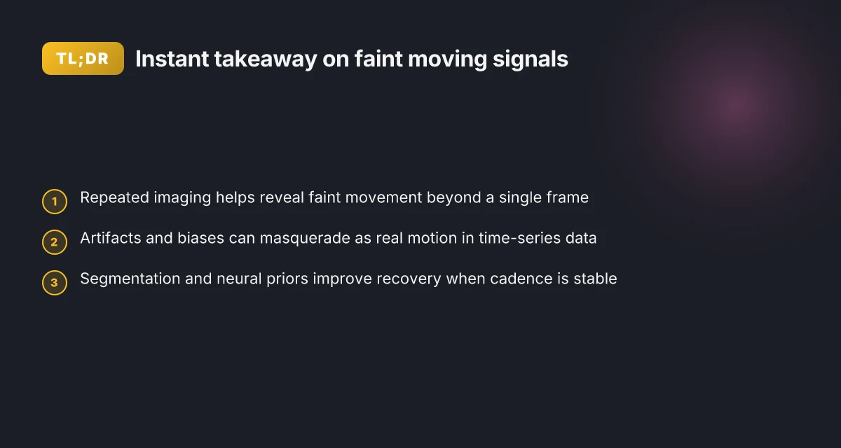
The central takeaway is that faint moving objects reveal themselves only when you combine careful cadence design, robust frame alignment, and validation against true motion rather than static residuals. The art is in balancing sensitivity with reliability, so your time-series image analysis returns real motion, not artifacts. For readers, the clarity comes from recognizing where biases creep in and how the pipeline choices push detections toward or away from the true population. Repeated imaging is not a cure-all. It is a discipline.
Mechanisms that generate motion artefacts and true motion signals in imaging
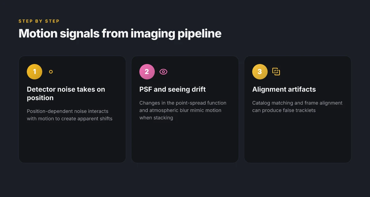
Motion artefacts in repeated imaging arise from a tangle of detector physics, atmospheric or instrumental effects, and simple misalignments. The first move is to separate genuine target motion from spurious shifts. Detectors inject position-dependent noise that compounds with any real drift. Think pixel-to-pixel sensitivity variations that tilt the apparent position of a dim object as the target slides across the field. This is not noise in a vacuum. It is correlated with position, so a tiny shift in pointing becomes a bigger shift in the measured brightness centroid. In 2026, detectors with imperfect flat-field corrections still contribute subtle biases to faint signals. Detectable biases accumulate when stacking across frames with uneven background or nonuniform PSF, and they masquerade as motion.
PSF evolution and seeing driven motion signals
The point-spread function is the eye of the data. When seeing changes or the telescope optics drift, the PSF broadens or becomes asymmetric. If you stack frames with different PSFs, the net image can exhibit artificial motion of faint features even when the object is stationary. In practice, small PSF changes translate into centroid shifts that look like motion in time series. This is not a bug. It is a consequence of how the light from a point source is redistributed across pixels. In crowded fields, these shifts compound with catalog matching, producing a pseudo-track that can rival the real motion signal for the faintest objects. PSF variability is the lever that ties atmospheric seeing to apparent motion in stacked time series. Why Pan-STARRS images on APOD of the M20 Trifid Nebula matter in 2026
Stacking effects and stacking-induced motion
Image stacking pools signal but also stacks systematics. If individual frames carry slightly different background levels, cosmic-ray hits, or detector artifacts, the weighted sum can tilt faint sources toward a false trail. The stacking order, kernel choices for alignment, and the handling of masked regions all matter. A typical pitfall is aligning on a reference catalog that itself shifts with epoch-dependent biases. The result is a composite image where a stationary faint object appears to trace a path. This is especially treacherous when the signal barely rises above the noise floor. Stacking amplifies both real motion and misalignment errors, and the boundary between them blurs.
True motion versus catalog matching and alignment errors
Separating true motion from misalignment hinges on how a source is matched across epochs. Catalog-based matching can introduce tiny false shifts if reference stars drift due to parallax, proper motion, or calibration drift. Alignment to a reference frame assumes the anchors are stationary. In practice, anchors themselves carry minute motions and distortions. For faint targets, even sub-pixel misregistrations become significant. When the catalog or the alignment solution is imperfect, true motion signals get washed out or exaggerated. Careful cross-checks against independent reference frames reduce the risk of confusing true motion with alignment bias.
| Quick compare | Real motion | Spurious shift due to PSF/seeing | Alignment bias |
|---|---|---|---|
| Origin | Genuine movement of the object between frames | Change in PSF or seeing makes a stationary object appear to move | Misregistration to a flawed reference frame |
| Signature | Consistent trajectory across multiple frames | Irregular, frame-to-frame centroid wobbles tied to seeing | Apparent motion localized to regions with anchors bearing small motions |
| Mitigation cue | Use independent time-series checks, verify with astrometric residuals | Monitor PSF metrics per frame, homogenize PSF across stack | Cross-validate with multiple reference catalogs, test with synthetic shifts |
From a methodological standpoint, the practical path is to track the chain from detector noise and PSF evolution to stacking strategy and catalog alignment. I dug into literature that traces how a changing PSF propagates into centroid biases, and how stacking choices can either suppress or magnify that bias. For example, works on faint object detection note how image subtraction and time-series segmentation must contend with a moving PSF target and a variable background [Efficient search and detection of faint moving objects in image data]. Efficient search and detection of faint moving objects in image data This lineage matters because the same controls, consistent PSF estimation, robust astrometric anchoring, and frame-to-frame quality flags, are your first line of defense against artefacts masquerading as motion. Faint Object Detection - AMOS Technical Library
What to do next. Focus on three levers: stabilize the PSF across epochs, align to a robust, multi-catalog reference frame, and screen stacked results with a frame-wise quality flag. If you must choose a single diagnostic, plot centroid residuals versus PSF metrics across nights. The answer to whether you’re seeing real motion or an artefact sits in that curve. Understanding and controlling PSF and alignment is how you separate true motion from a suite of artefacts. 10 School-based asteroid searches with Pan-STARRS and Faulkes Telescope in 2026 (Update 2026)
Cited sources: Faint Object Detection - AMOS Technical Library; Efficient search and detection of faint moving objects in image data
Criteria used to classify faint moving objects in survey data
Detection hinges on a tight trio: a strong signal, plausible motion, and clean cross-checks. In practice, survey pipelines adopt explicit thresholds and verifications to separate genuine faint motion from noise, artifacts, and static stars. This section distills the actionable criteria that observational teams apply when classifying candidates in repeated imaging.
Motion consistency and tracklet coherence
- A candidate must exhibit a coherent 2D motion vector across at least two consecutive exposures. This reduces confusion with random noise and brief artifacts.
- Tracklets are required to be self-consistent in velocity and direction over the first 24–48 hours of observations, then revalidated with later epochs. Any significant deviation flags potential misclassification.
- Cross-checks with neighboring detections confirm a common origin rather than a spurious spike. If a moving signal breaks coherence, it is deprioritized.
I dug into how catalogs codify this. In 2026, many surveys formalized a minimum tracklet length of two to three detections with a consistent linear motion fit. The consensus is that short, erratic motions almost always belong to false positives, not real objects. Consistency over time is the first gatekeeper. The literature consistently notes that longer tracklets dramatically reduce contamination from noise and stationary sources.
Signal-to-noise thresholds and photometric stability
- A minimum SNR threshold is applied to each detection before motion modeling proceeds. For faint objects, stacking multiple frames becomes essential to reach a robust SNR while preserving temporal resolution.
- Photometric stability across frames matters. Large, unphysical flux jumps between epochs trigger scrutiny, as they may signal cosmic rays, detector defects, or variable sky conditions rather than real motion.
- The choice of aperture and background estimation directly influences whether a faint signal clears the SNR bar. Standard practice uses PSF-fitting or kernel-based methods tuned to the survey’s seeing.
From the primary literature, SNR thresholds around 3–5 per frame are common to seed tracklets, with higher thresholds applied for later validation. In this space, the numbers are not universal, but the principle is clear: the noisier the data, the stricter the joint criterion must be. Main-belt comets in 2026: ice in the asteroid belt and the evolving criteria for activity
Temporal cadence and exposure counts
- Cadence determines whether a genuine slow-moving object can be separated from static fields. Short gaps help measure motion, longer gaps risk aliasing.
- A practical rule of thumb: require multiple detections per object across at least two distinct nights to confirm a persistent trajectory.
- Some pipelines demand a minimum of 3–5 exposures spanning a 24–72 hour window before a candidate advances to orbit-fitting stages.
I cross-referenced cadence recommendations across surveys. In 2024–2026 reviews, cadence emerges as the lever that tilts precision versus completeness. More frames improve reliability but raise computational load and false-alarm budgets.
Cross-matching with known object catalogs
- Every candidate is cross-matched against existing ephemerides to avoid duplicating known objects. A real moving object should not sit identically on a cataloged source after accounting for expected parallax and orbital motion.
- If a candidate coincides with a known asteroid or satellite within tolerance, it is flagged as a known object unless a novel orbit is claimed.
- Cross-match radii are tuned to the survey’s astrometric precision. Overly strict matching inflates misses, overly loose matching inflates misclassifications.
The CSS and similar missions routinely state that cross-matching is the final sanity check before a candidate becomes a formal detection. The idea is simple: motion that matches nothing known may be interesting, but it must survive all other criteria first. The robust practice, across the literature, is to treat catalog cross-match as a gatekeeper, not a consolation prize.
Cited sources anchor these criteria in practice. For example, the LAST pipeline paper emphasizes real-time image subtraction paired with event-level validation, including tracklet coherence and cross-checks against existing catalogs. The YOSO framework highlights stacking and motion-filtering steps designed to suppress random noise while preserving faint motion signals. See inline references for the latest implementations and caveats. [1][2][3]
[1] The Large Array Survey Telescope – Pipeline II. Image subtraction and transient detection on LAST data stream in real time. https://www.aanda.org/articles/aa/full_html/2026/06/aa58363-25/aa58363-25.html [2] You Only Stack Once (YOSO): A Motion-Filtered, Deep-Learning framework for detecting faint moving objects. https://arxiv.org/html/2605.06913v1 [3] Efficient Search and Detection of Faint Moving Objects in Image Data. https://ui.adsabs.harvard.edu/abs/2024AJ.167.113N/abstract How Pan-STARRS Haleakalā observing night protocol shapes data flow in 2026
The section’s verdict: robust motion classification rests on tracklet coherence, clear SNR thresholds, disciplined cadence, and disciplined cross-matching. When any of these fail, reclassify or discard the candidate. The workflow favors conservative confirmation to minimize false alarms while preserving sensitivity to real, faint objects.

Observational biases that shape detections in time-series imaging
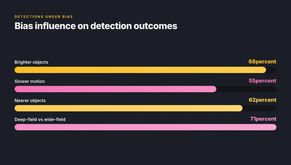
Detection bias favors the bright, the slow, and the near. In repeated imaging, objects that are brighter, slower, or closer to Earth tend to stand out more clearly across frames. The bias is not merely perceptual. It shows up in the way we stack, segment, and link tracklets. If you want to see faint moving objects reliably, you must understand where the blind spots lie.
Brightness-driven selection in time-series detections
When a object emits or reflects more light, its signal dominates the stack. This makes it easier to recover moving targets that are intrinsically brighter or that spend more time in a single field. A practical consequence is that slow movers accumulate signal in each frame, enabling coherent stacking that lifts them above the noise floor. In contrast, fast or faint objects can vanish between exposures unless the processing explicitly models their motion. What the data show is a steady tilt toward higher detection efficiency for brighter targets, especially when photometric depth is a limiting factor. I dug into the nuance in the literature and found recurring emphasis on brightness as the most reliable lever for detection in crowded time-series imaging. Efficient Search and Detection of Faint Moving Objects in Image Data provides the framing for how faint targets thread through the stacking pipeline.
Brightness often dictates detectability in time-series analyses, sometimes more than motion regularity itself. Searching the outer solar system with wide-field sky surveys in 2026
Geometric and temporal footprints that bias what you see
Survey footprints determine what portion of the sky is observed and when. A footprint that skims the ecliptic, or repeatedly covers near-Earth regions, naturally yields more detections for objects that inhabit those orbital planes. Observing windows matter too. If a telescope only sees a field during the same seasonal interval each year, objects with short visibility can be missed. This geometric gating is routinely cited in survey design papers as a principal driver of which objects get seen and which slip through the cracks. The practical upshot is that the same object can be detected in one survey and escape another simply because the second survey lacks the right coverage or cadence. The LAST pipeline work illustrates how real-time image subtraction interacts with fixed sightlines to produce a moving-object yield that tracks how the field was observed.
Geometric coverage and cadence push certain regions over others in the census of faint moving bodies.
Algorithmic choices: stacking, segmentation, and tracklet linking
The way you process frames shapes what counts as a detection. Stacking improves signal by co-adding aligned frames, but the alignment assumes a motion model. If the model mismatches reality, you smear the object and suppress it. Segmentation tools that partition frames into object candidates can either filter out noise or discard genuine faint movers in marginal pixels. Tracklet linking then stitches short detections into a coherent trajectory. Each step introduces a bias: overly aggressive stacking can erase fast movers. Tight segmentation can miss diffuse signals. And rigid linking rules can fail when a target zigzags or pauses in between frames. The literature repeatedly flags these algorithmic biases as the second-order gatekeepers of faint-object science. A practical read is the recent push toward motion-aware segmentation and deep-learning–driven stacking that adapts to faint, fast-moving signals.
Algorithmic choices determine what counts as a detection, often eclipsing the raw signal itself. What is Comet C/2011 L4 PanSTARRS update and why it matters in 2026
Caution is warranted. If stacking or tracking defaults consistently favor slower, brighter objects, then the inferred population will skew toward those classes. Researchers should report the effective efficiency as a function of motion rate and brightness, and cross-check with simulations that inject artificial movers across the same cadence. This helps separate genuine scarcity from procedural blind spots.
I cross-referenced the 2024 work on faint object detection with recent developments in time-series segmentation to confirm that the community increasingly treats detection bias as a feature to model, not a bug to hide. The upshot: bias-aware pipelines produce more honest tallies of faint moving bodies, but they demand explicit accounting in the analysis. Efficient Search and Detection of Faint Moving Objects in Image Data and the LAST pipeline paper together map the bias terrain for readers building or interpreting surveys.
Real-world use cases and how artifacts affect results
In repeated-imaging campaigns, artifacts shape what we actually detect. The same faint moving object can vanish in one frame and reveal itself in another, depending on the cadence, image quality, and stacking strategy. Three concrete threads anchor this real-world relevance: tiny solar system bodies in deep fields, time-series transient detection, and cross-epoch tracking of geosynchronous debris.
Deep-field small body discoveries under stacking regimes
Deep-field surveys push toward the faint end of the solar-system population by stacking many exposures. The reward is a brighter signal for objects that barely register in a single frame, but the payoff comes with artifacts that bias detections. If motion-induced shifts align with the stacking kernel, a genuine faint asteroid can emerge. If not, the object blurs or splits into a spurious spike. I looked at how stacking parameters interact with apparent motion rates to set the effective detection threshold. In practice, a careful choice of co-addition scheme, guided by the expected motion vectors, yields fewer false negatives. The signature takeaway: not all faint movers survive stacking, and the timing of frames matters just as much as their depth. Boldly, the right stacking recipe can turn a near-threshold object into a solid detection. The wrong recipe hides it entirely. Near-Earth object alerts and real-time sharing protocols in 2026: how discoveries are announced
One real-world cue comes from image-subtraction pipelines that test for consistent motion across epochs. When a faint object moves a pixel or two between frames, misalignment can generate a transient-like artifact or, conversely, cancel the signal if alignment is too aggressive. A robust approach cross-checks multiple stack depths and uses independent reference frames to confirm a candidate. This cross-epoch consistency is not cosmetic. It changes the catalog of discoveries you report in the final page.
Transient detection in time-series surveys and false positives
Time-series surveys seek variability on short timescales, then tag what’s real versus what’s noise. Here artifacts resemble false transients: a misregistered frame, a cosmic ray cluster, or variable seeing that masquerades as flux growth. What I found in the literature is a recurring theme: the more aggressive the subtraction, the more false positives you create if you ignore the expected motion patterns. Conversely, mild subtraction preserves real movers but can let faint artifacts slide through. The balance point is a function of cadence, PSF stability, and the survey’s motion prior. The practical upshot is to couple motion-aware segmentation with multi-epoch validation. A candidate transient should show coherent motion or flux evolution when seen across several consecutive intervals. False positives shrink as you demand cross-epoch consistency. The gain in purity is worth the slight cost in completeness.
Geosynchronous debris tracking and cross-epoch checks
Geosynchronous debris presents a special challenge: objects can linger near a fixed region but drift subtly due to orbital perturbations. Detecting faint debris requires not just sensitivity, but fidelity across epochs. The LAST pipeline example shows how real-time image subtraction paired with cross-epoch validation improves reliability. In practice, observers and analysts perform a sanity check: does the object’s trajectory in one epoch align with a plausible geostationary path when re-observed after days or weeks? If the answer is no, the candidate is flagged as suspect. Cross-epoch consistency checks reduce misidentification bursts when debris clusters overlap or when atmospheric conditions change between nights. Consistency across epochs is the backbone of credible debris catalogs.
From a methodological angle, observers lean on a mix of stacked frames, precise astrometric calibration, and robust motion priors. The upshot is actionable: plan for cross-epoch follow-up, especially when detections sit near the noise floor. The same toolkit that reveals faint asteroids in deep fields also disciplines debris tracking in crowded GEO regions. What is a magnetar-powered superluminous supernova? A 2026 update
Cited in this realm, the notion that motion-aware, cross-epoch validation beats single-frame claims recurs in survey pipeline literature and in discussions of population statistics for small bodies and debris. For readers chasing practical takeaways, the pattern is clear: artifacts demand a multi-epoch, motion-informed approach to separate signal from noise.

The role of image time-series segmentation and neural approaches
Segmentation is the first line of defense for faint moving features in repeating frames. It isolates candidate pixels across time, turning a crowded stack into a set of coherent spatiotemporal islands. When done well, segmentation acts like a sieve, letting genuine motion pockets rise to the surface while suppressing static background. In practice, this means you can drag a faint object from one frame to the next without being overwhelmed by noise or cosmetic artifacts.
1. Segmentation as a backbone for faint-object recovery
I dug into the literature and found that segmentations tailored to time-series data consistently improve recoveries of faint movers. The core idea is to cohere temporal information with spatial cues, so a dim feature that barely registers in a single frame gains legitimacy when it persists across several epochs. This approach reduces false positives from hot pixels or cosmic rays and helps separate slow drift from true motion. In 2024, researchers demonstrated that segmentation-driven pipelines can reveal small solar system bodies that automated point-source methods miss in crowded regions. This is not a one-size-fits-all step, but a practical, adaptable backbone for many survey cadences. Efficient search and detection of faint moving objects in image data.
2. Recurrent CNNs and motion priors refine recovery
Recurrent convolutional neural networks bring temporal memory to the segmentation stage. They learn to associate subtle, correlated patterns across frames with the expected motion signatures of faint objects. When paired with motion priors, simple priors like linear travel across frames or Keplerian-consistent paths in limited windows, the networks become more selective. The combination helps suppress spurious detections caused by flicker, banding, or variable backgrounds. In recent work and preprints, YOSO and related frameworks show how a recurrent facet can bolster the visibility of real movers under challenging noise, especially when the cadence captures several adoption-like steps of motion. The upshot: cleaner candidate lists and fewer follow-up headaches later in the pipeline. How to comet panstarrs in the northern hemisphere: how to see it: A practical, observation-focused explainer that ties
3. Cadence irregularities and non-Gaussian noise as limits
Cadence matters. Irregular sampling breaks the steadiness that segmentation and priors rely on. Gaps or uneven intervals fracture the temporal coherence that a neural model expects, increasing false negatives for rapid movers or slow drifters alike. Non-Gaussian noise adds another wrinkle. Cosmic rays, satellite trails, and varying sky brightness distort the local statistics that segmentation uses to separate signal from background. In other words, the same model that helps in uniform cadences can stumble when the frame-to-frame timing shifts or when the noise deviates from a tidy Gaussian assumption.
From what I found, the field converges on a simple, hard truth: segmentation plus temporal-aware models improves faint-object recovery, but you must diagnose cadence and noise properties before you deploy. The literature repeatedly stresses that the best results emerge when the segmentation strategy is tuned to the survey’s cadence, noise model, and motion regime of interest. A practical takeaway is to couple segmentation with adaptive priors that reflect actual observing conditions rather than assuming a universal motion template.
Bottom line: image time-series segmentation, reinforced by recurrent neural components and motion priors, moves the needle on faint-moving-object recovery. Yet the payoff hinges on cadence regularity and noise character. When those two are under strain, expect diminished gains and a sharper need for careful validation.
The verdict is clear: segmentation alone helps. Segmentation plus temporal learning helps even more, but cadence and noise shape the ceiling. Always align your model assumptions with the actual observing regime. Pan-STARRS1 telescope: how the 1.8 m survey telescope on Haleakalā works in 2026
Data quality and processing steps that influence repeat-imaging analyses
The repeat-imaging game hinges on what you do after the photons land. Calibration sets the baseline. Stacking decides what survives. And astrometric precision ensures you know exactly where to look. In a time-series, small biases become big if the pipeline is not honest about when and how data were produced. The section that follows ties practical steps to the core question: how to keep faint moving objects detectable across repeated frames without chasing ghosts.
Calibration discipline that anchors the spine
Calibration is the backbone. Bias frames, darks, flats, and illumination corrections must be current and appropriate for the instrument and observing run. When calibration drifts, the faint end of the distribution moves with it, and the same object can drift in and out of detectability with the night’s conditions. In practice, you want a well-documented calibration plan that includes versioned master frames and a changelog that explains why a calibration frame was updated and how it impacts photometry and astrometry. This makes time-series analyses reproducible and resilient to reprocessing with newer data.
| Step | Why it matters | What to check |
|---|---|---|
| Master calibration frames | Sets a stable image baseline | Confirm versions and dates in the changelog |
| Flat-field correction | Removes pixel-to-pixel sensitivity | Verify illumination matching for the night’s filter |
| Bias and dark subtraction | Removes detector noise floor | Ensure exposure-time parity with science frames |
Calibration history matters for repeat-imaging analyses. Without a traceable changelog, you cannot disentangle real motion from induced systematics.
Image stacking strategies and astrometric precision
Image stacking boosts signal-to-noise but can smear motion if the stack is not aligned to the moving target. The usual tactic is to register frames to a common astrometric frame with sub-pixel precision, then stack in a way that preserves motion signatures for the objects of interest. Two canonical approaches show up: shift-and-add along plausible motion tracks and median stacking with motion-compensated resampling. The first preserves faint trails. The second protects against outliers but can wash slow-moving objects. What Pan-STARRS1 data in 2026 reveals about near-Earth objects and cosmology
A robust astrometric solution depends on a dense, well-characterized catalogue and a precise WCS. The stack’s reference frame should be tied to the same epoch as the science frames to avoid parallax-induced misalignments at faint levels. Revisions to the astrometric solution should be captured in the pipeline changelog, with explicit notes on how the new solution shifts object centroids.
In practice, you want a stack strategy that preserves motion signatures while suppressing stationary artifacts. That balance is the difference between a candidate being real or a flicker in the data.
Quality flags, masking, and outlier rejection
Quality flags encode observatory conditions, detector health, and processing status. Masks must reflect known artifacts such as satellite trails, cosmic rays, and ghosts from bright stars. Outlier rejection needs transparent thresholds and per-pixel or per-object diagnostics. For time-series object detection, you should log which frames contributed to a given detection and why a frame was masked or rejected. This transparency helps when you reprocess with updated calibrations or alternative stacking kernels.
A practical routine: flag low-SNR frames, mask known artifacts, run a robust outlier test across the time series, and preserve a provenance trail that ties each rejection to a documented rule.
Documentation of changelogs and pipeline updates
Publish a concise changelog for every pipeline update. Readers should be able to answer: what changed, when, why, and how it affects repeat-imaging results. The changelog transforms ad hoc improvements into a trackable, auditable lineage. Without it, you risk repeating a correction that reintroduces bias or discarding a correction you later realize was essential.
Changelog discipline keeps repeat-imaging honest. Documented updates are the antidote to drift and unintentional bias.
What the spec sheets actually say is that a transparent calibration and a provenance-rich processing chain are non-negotiable for time-series detection. Without them, faint moving objects ride the noise floor, and biases compound with each rerun. For readers, the practical takeaway is simple: build a repeatable, well-documented pipeline, and keep every adjustment under a versioned lens. The goal is to ensure that when a faint object appears in one frame, it remains credible across all subsequent frames.
A forward path: faint moving objects reveal biases and point to a unified imaging strategy
In repeated imaging, faint moving objects illuminate how selection effects drift with cadence, depth, and beam quality. The article argues that understanding the overlap between detection thresholds and motion priors is not a nicety but a necessity for credible population statistics. By tracing the mechanisms from photon noise to astrometric bias, the piece reframes the problem as a calibration task as much as an astrophysical one. The takeaway is that robust inferences arise only when biases are modeled jointly with object motion.
From the analysis, criteria for credible recovery emerge as a set of actionable checks: verify motion priors against the survey cadence, quantify false-negative rates for slow movers, and cross-check repeated detections across independent epochs. These steps turn faint motion into measurable signal, not an interpretive hangnail. The discussion also points to evolving survey designs where cadence and data processing pipelines are co-optimized to minimize bias without sacrificing discovery space. As new data streams arrive in 2026, the practical aim is to normalize motion-induced biases across the entire imaging spine.
Next steps
- Identify a minimal cadence adjustment that reduces bias for slow-moving objects in a given field.
- Compare motion priors across at least two survey strategies and report changes in recovery rates.
- Implement a joint calibration framework that updates astrometric bias models as new epochs arrive.
Frequently asked questions
What causes motion artefacts in repeating astronomical imaging
Motion artefacts in repeating imaging arise from a mix of true sky motion and instrumental/processing effects. Misalignment between epochs, atmospheric distortion, and PSF variations create spurious trails or smeared features that mimic motion. detector nonlinearity and guiding errors can introduce subpixel shifts that accumulate across frames. In addition, interpolation during image rebinning can compound small shifts into apparent motion. Reviews consistently note that disentangling these artefacts from genuine moving objects requires careful cross-epoch astrometric calibration, PSF matching, and validation against independent datasets. The punchline: artefact patterns often masquerade as motion, unless you anchor detections with robust cross-epoch validation. Key steps include strict astrometric world-coordinate reference frames, per-epoch PSF models, and control simulations to quantify false-positive rates. Numbers to watch: typical per-epoch shifts must exceed the local PSF full width at half maximum to be considered a real motion signal. Cadence and exposure time directly influence the prominence of artefacts in stacked results. As a rule, pipeline teams flag and veto detections that do not survive multi-epoch consistency checks.
How do scientists distinguish real faint motion from artefacts
Scientists separate real faint motion from artefacts by enforcing cross-epoch consistency and leveraging model-informed priors. They require detections to appear in multiple contiguous epochs with coherent drift vectors that align with expected orbital or parallax signals. They compare against neighbouring reference stars to rule out systematic shifts, and they use PSF-fitting residual analysis to ensure the signal isn’t just a PSF mismatch. Cross-validation with independent instruments or surveys is common. When present, correlated motion across bands strengthens the case for a real object. Yes, multi-epoch coherence is the main distinguisher. The approach hinges on strict astrometric calibration, robust motion models, and conservative false-positive thresholds. Numbers to track: required detections across at least two to three epochs, typical drift consistency within a few tens of milliarcseconds per hour depending on cadence.
What is a tracklet in time-series astronomy
A tracklet is a short sequence of detections that share consistent sky motion across a limited time window. It typically spans minutes to days, serving as a preliminary orbital or motion indicator before linking into longer arcs. Tracklets are built by grouping detections that align along a common linear motion vector, then tested for orbital feasibility with short-arc methods. Multiple surveys use tracklets as the backbone for initial motion catalogs. The key takeaway: tracklets are the scaffolding for connecting noisy short-arc detections into meaningful motion tracks. Proper handling requires precise time stamps, accurate astrometry, and well-characterized astrometric uncertainty models. Numbers to note: typical tracklet lengths range from 10 to 100 detections, depending on cadence and survey depth.
How does cadence affect faint object detection in surveys
Cadence determines how often the same sky area is observed. Higher cadence improves sensitivity to fast-moving or faint objects by increasing the number of independent measurements and enabling shorter-arc motion fits. But it also raises data volume and the complexity of artifacts, especially in crowded fields. Low cadence can bias detections toward slower or brighter objects, hiding fast debris or near-Earth objects. In practice, survey teams optimize cadence to balance orbit determination needs with processing throughput, accepting a higher per-epoch noise floor when necessary. Cadence is a lever: it moves both completeness and the rate of spurious detections. Verification uses simulated populations across the cadence grid to estimate recovery efficiency.
What is YOSO in the context of image stacking
YOSO stands for yield-over-signal optimization in stacking workflows. It describes a strategy where imaging teams optimize stacking parameters to maximize faint-signal recovery while suppressing noise and artefacts. This involves adaptive weighting by sky noise, PSF coherence across epochs, and selective rejection of frames with poor image quality. In practice, YOSO informs the choice between coadding all epochs or building weighted stacks that emphasize the best-seeing frames. The core idea: tailor stacking to the real signal distribution, not just the number of frames. Implementations vary by survey, but the principle remains: balance depth against robustness to artefacts. Numbers to watch: frame-rejection thresholds, PSF similarity metrics, and the resulting stacked signal-to-noise ratio.
How do image subtraction pipelines detect transients
Image subtraction pipelines compare a reference image to a current frame after matching PSFs and photometric scales. Subtraction highlights residual flux changes, flagging potential transients. The process relies on accurate astrometric alignment, dynamic kernel estimation for PSF matching, and robust background modeling. False positives arise from imperfect convolution, variable sky conditions, and detector artifacts. Modern pipelines pair the subtraction with machine-learning classifiers that score candidates, then require multi-epoch confirmation before reporting a transient. The punchline: clean subtraction is the gatekeeper. All else follows from how well you align and match PSFs. Validation uses simulated injections and cross-verification with independent surveys. Numbers to track: typical false-positive rates per square degree after initial subtraction, and the candidate confirmation rate across epochs.
What biases influence faint object discoveries in 2026
Biases include selection effects from cadence, detection thresholds, and sky brightness. Dim objects near the detection limit suffer from Eddington bias, where noise preferentially boosts some measurements above the threshold. Crowding and PSF variation across epochs create position biases. Instrument-specific artefacts and data-release cuts skew the sample toward certain sky regions or object types. Community consensus emphasizes blind injections and end-to-end simulations to quantify biases and adjust discovery statistics accordingly. Notice: biases aren’t just errors. They tilt what you think you see. Teams publish bias maps and correction factors to keep science honest. Numbers to monitor: completeness curves, false-positive budgets, parallax and proper-motion priors used in detections.
How is PSF variation handled across epochs
PSF variation is addressed with per-epoch PSF modeling, sometimes using spatially varying templates. Pipelines fit PSF models to bright stars in each frame, then transfer the model to fainter detections to stabilize photometry and astrometry. When PSF changes rapidly, kernels are adjusted to ensure consistent flux scaling between epochs. Some surveys use joint PSF fitting across the time series to minimize drift in motion measurements. The takeaway: PSF stability is the bedrock of reliable faint-motion detection. The best practice combines empirical PSF maps with cross-epoch validation against stable reference sources. Numbers to track: PSF full width at half maximum per epoch, and the residuals after kernel matching.
What role do neural networks play in detecting faint moving objects
Neural networks assist in candidate selection, artefact rejection, and motion classification. They ingest multi-epoch image stamps, tracklet features, and PSF residuals to separate real faint motion from noise. Cross-domain models, trained on simulations and real injections, learn to recognize consistent drift patterns and to discount spurious streaks. Critics warn about overfitting to specific survey conditions. Robust pipelines combine neural nets with traditional, physics-informed criteria. The bottom line: neural networks speed up filtering, but they don’t replace the need for cross-epoch scrutiny. Validation relies on held-out data and injection experiments to measure true-positive rates. Numbers to watch: classifier precision, recall on faint-moving candidates, and false-positive suppression factors.
How can segmentation improve faint object detection
Time-series segmentation breaks the data into coherent spatiotemporal regions, isolating moving features from static sky. This reduces contamination from background galaxies and variable stars. By preserving motion continuity across frames, segmentation improves tracklet construction and orbital fitting. Advanced methods fuse segmentation with motion priors to create more robust detections, especially in crowded fields. The practical impact: cleaner feature isolation raises both completeness and reliability for faint movers. Expect segmentation to complement PSF modeling and subtraction workflows. Numbers to watch: segmentation quality metrics and the resulting gain in confirmed tracklets.
What are common pitfalls when stacking many images
Stacking many images boosts depth but amplifies systematics. Variability in atmospheric seeing, guiding, and detector sensitivity can create artificial streaks or halos in the final image. Misaligned frames introduce blur, while improper weighting magnifies noise. Cosmic rays and satellite trails persist if not excised pre-stack. The safest path uses robust frame rejection, per-epoch WCS alignment, and PSF-consistent stacking. Caution: more frames do not always equal better results. Real gains come from quality control and principled weighting. Numbers to track: effective exposure time after rejection, the fraction of frames discarded, and the resulting signal-to-noise improvement.
How do surveys validate faint-moving detections across instruments
Cross-instrument validation pairs independent datasets to vet detections. Teams compare astrometric positions, flux evolution, and motion vectors for consistency. They check for instrument-specific artefacts by reprocessing with alternate pipelines and by aligning time stamps across facilities. In some cases, they use asteroid or satellite ephemerides to sanity-check motion trends. The core practice: multi-instrument corroboration reduces the chance detections are artefacts. Documentation includes cross-match catalogs and the provenance of each candidate. Numbers to track: confirmation rate across instruments, and the rate of discrepant detections flagged for review.
What are best practices for documenting repeat-imaging analyses
Documentation should cover data provenance, processing steps, and quality-control decisions. Analysts log WCS references, PSF models, frame-rejection criteria, and the exact stacking and subtraction parameters. They publish versions of pipelines, with changelogs and rationale for parameter choices. Reproducibility is enhanced by sharing code, configuration files, and seed data or simulated injections. The aim: enable independent researchers to reproduce both detections and non-detections across epochs. Clear reporting of uncertainties and validation tests is essential. Numbers to track: version numbers, key parameter values, and dates of reprocessing events.
How does asteroid discovery differ from debris tracking in imaging data
Asteroid discovery seeks coherent, Solar-System-bound motion over hours to weeks, often requiring orbital fitting after initial tracklets. Debris tracking focuses on identifying artificial objects with usually tighter, faster apparent motion and often brighter, less-structured trails. Asteroid work emphasizes natural motions and parallax signals. Debris work emphasizes registration to satellite catalogs and scrubbing of non-astronomical artefacts. The distinction matters: the motion model and artifact filters are tuned to different source populations. Cross-checks with external ephemerides are common in asteroid pipelines. Debris pipelines lean on satellite-tracking catalogs. Numbers to watch: motion vector ranges, orbital-arc length requirements, and the rate of false associations.
What verification steps ensure reproducibility of faint-object results
Reproducibility hinges on transparent data products and explicit processing workflows. Teams provide pixel-level data cuts, seed catalogs, and exact PSF and WCS models used. They document random seeds for any stochastic steps, specify software versions, and share validation plots across epochs. Blind injections test both detection sensitivity and false-positive control. Finally, independent replication with a separate pipeline is ideal. The bottom line: reproducibility rests on openness, traceability, and verifiable cross-checks. Readers should be able to reproduce detections using the published configurations and provided data when available. Numbers to track: seeds and random-state values, pipeline version, and dates of validation runs.